|
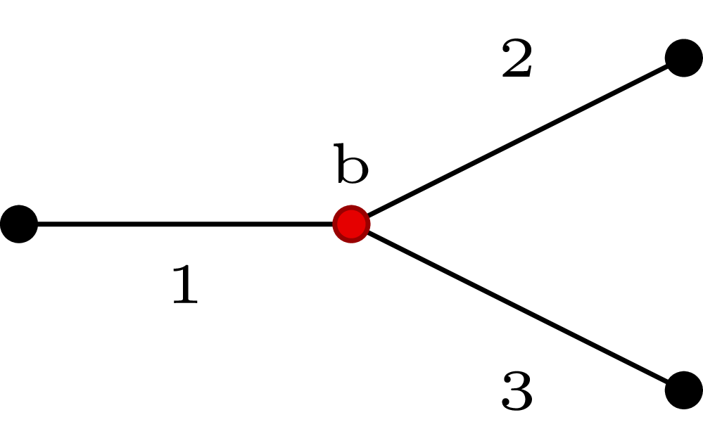
In a bifurcation, there is a parent vessel (indicated as 1 in the figure) and two daughter vessels (2 and 3).
The bifurcation is solved by imposing the conservation of mass and of static pressure at the bifurcation node \(b\). Three additional relations are obtained by extrapolating the three outgoing characteristics. The solution process is the same described for the conjunction case.
\(U\) and \(F\) vectors read \[
U = \{U_i\} = \left\{ \begin{array}{c}
u_1 \\
u_2 \\
u_3 \\
A_1^{1/4} \\
A_2^{1/4} \\
A_3^{1/4}
\end{array} \right\} , \quad i =1, ..., 6,
\] \[
F = \left\{f_i \right\} =
\begin{cases}
U_1 + 4k_1U_4 - W_1^* = 0, \\
U_2 - 4k_2U_5 - W_2^* = 0, \\
U_3 - 4k_3U_6 - W_3^* = 0, \\
U_1U_4^4 - U_2U_5^4 - U_3U_6^4 = 0, \\
\beta_1 \left(\tfrac{U_4^2}{A_{01}^{1/2}} -1 \right) -
\beta_2 \left(\tfrac{U_5^2}{A_{02}^{1/2}} -1 \right) = 0, \\
\beta_1 \left(\tfrac{U_4^2}{A_{01}^{1/2}} -1 \right) -
\beta_3 \left(\tfrac{U_6^2}{A_{03}^{1/2}} -1 \right) = 0, \\
\end{cases}
\] and the Jacobian reads \[
J = \left[ \begin{array}{cccccc}
1 & 0 & 0 & 4k_1 & 0 & 0 \\
0 & 1 & 0 & 0 & -4k_2 & 0 \\
0 & 0 & 1 & 0 & 0 & -4k_3 \\
U_4^4 & -U_5^4 & -U_6^4 & 4U_1 U_4^3 & -4 U_2 U_5^3 & -4U_3 U_6^3 \\
0 & 0 & 0 & 2\beta_1 U_4/A_{01}^{1/2} &
-2\beta_2 U_5/A_{02}^{1/2} & 0 \\
0 & 0 & 0 & 2\beta_1 U_4/A_{01}^{1/2} &
-2\beta_2 U_5/A_{02}^{1/2} & 0 \\
\end{array} \right].
\] The solution is performed by solveBifurcation and follows the same procedure of solveConjunction function. Refer to conjunctions.jl documentation for further informations.
|
|
|
function solveBifurcation
v1 |
::Vessel data structure for the parent vessel. |
v2 |
::Vessel data structure for the first daughter vessel. |
v3 |
::Vessel data structure for the second daughter vessel. |
|
function solveBifurcation(v1 :: Vessel, v2 :: Vessel, v3 :: Vessel)

  #Unknowns vector
  U = [v1.u[end],
       v2.u[ 1 ],
       v3.u[ 1 ],
       sqrt(sqrt(v1.A[end])),
       sqrt(sqrt(v2.A[ 1 ])),
       sqrt(sqrt(v3.A[ 1 ]))]

  #Parameters vector
  k1 = sqrt(0.5*3*v1.gamma[end])
  k2 = sqrt(0.5*3*v2.gamma[ 1 ])
  k3 = sqrt(0.5*3*v3.gamma[ 1 ])
  k = [k1, k2, k3]

  W = calculateWstarBif(U, k)
  J = calculateJacobianBif(v1, v2, v3, U, k)
  F = calculateFofUBif(v1, v2, v3, U, k, W)

  #Newton-Raphson
  nr_toll_U = 1e-5
  nr_toll_F = 1e-5

  while true
    dU = J\(-F)
    U_new = U + dU

    if any(isnan(dot(F,F)))
      println(F)
      @printf "error at bifurcation with vessels %s, %s, and %s \n" v1.label v2.label v3.label
      break
    end

    u_ok = 0
    f_ok = 0
    for i in 1:length(dU)
      if abs(dU[i]) <= nr_toll_U || abs(F[i]) <= nr_toll_F
        u_ok += 1
        f_ok += 1
      end
    end

    if u_ok == length(dU) || f_ok == length(dU)
      U = U_new
      break
    else
      U = U_new
      W = calculateWstarBif(U, k)
      F = calculateFofUBif(v1, v2, v3, U, k, W)
    end
  end

  #Update vessel quantities
  v1.u[end] = U[1]
  v2.u[ 1 ] = U[2]
  v3.u[ 1 ] = U[3]

  v1.A[end] = U[4]*U[4]*U[4]*U[4]
  v2.A[ 1 ] = U[5]*U[5]*U[5]*U[5]
  v3.A[ 1 ] = U[6]*U[6]*U[6]*U[6]

  v1.Q[end] = v1.u[end]*v1.A[end]
  v2.Q[ 1 ] = v2.u[ 1 ]*v2.A[ 1 ]
  v3.Q[ 1 ] = v3.u[ 1 ]*v3.A[ 1 ]

  v1.P[end] = pressure(v1.A[end], v1.A0[end], v1.beta[end], v1.Pext)
  v2.P[ 1 ] = pressure(v2.A[ 1 ], v2.A0[ 1 ], v2.beta[ 1 ], v2.Pext)
  v3.P[ 1 ] = pressure(v3.A[ 1 ], v3.A0[ 1 ], v3.beta[ 1 ], v3.Pext)

  v1.c[end] = waveSpeed(v1.A[end], v1.gamma[end])
  v2.c[ 1 ] = waveSpeed(v2.A[ 1 ], v2.gamma[ 1 ])
  v3.c[ 1 ] = waveSpeed(v3.A[ 1 ], v3.gamma[ 1 ])

end
|
|
function calculateWstarBif \(\rightarrow\) W::Array{Float, 1}
U |
::Array junction unknown vector. |
k |
::Array junction parameters vector. |
| Riemann invariants are computed starting from unknown and parameters vectors as \[
W_1 = u_1 + 4c_1, \quad W_2 = u_2 - 4c_2, \quad W_3 = u_3 - 4c_3.
\] |
W |
::Array containing outgoing characteristics from the three vessels. |
|
function calculateWstarBif(U :: Array, k :: Array)

  W1 = U[1] + 4*k[1]*U[4]
  W2 = U[2] - 4*k[2]*U[5]
  W3 = U[3] - 4*k[3]*U[6]

  return [W1, W2, W3]
end
|
|
function calculateFofUBif \(\rightarrow\) F::Array
b |
::Blood data structure. |
v1 |
::Vessel parent vessel data structure. |
v2 |
::Vessel first daughter vessel data structure. |
v3 |
::Vessel second daughter vessel data structure. |
U |
::Array junction unknown vector. |
k |
::Array junction parameters vector. |
W |
::Array outgoing characteristics array. |
| \(F\) array is computed by imposing the conservation of mass and static pressure at bifurcation node. \(F\) reads \[
F = \left\{f_i \right\} =
\begin{cases}
U_1 + 4k_1U_4 - W_1^* = 0, \\
U_2 - 4k_2U_5 - W_2^* = 0, \\
U_3 - 4k_3U_6 - W_3^* = 0, \\
U_1U_4^4 - U_2U_5^4 - U_3U_6^4 = 0, \\
\beta_1 \left(\tfrac{U_4^2}{A_{01}^{1/2}} -1 \right) -
\beta_2 \left(\tfrac{U_5^2}{A_{02}^{1/2}} -1 \right) = 0, \\
\beta_1 \left(\tfrac{U_4^2}{A_{01}^{1/2}} -1 \right) -
\beta_3 \left(\tfrac{U_6^2}{A_{03}^{1/2}} -1 \right) = 0, \\
\end{cases}
\] |
Total pressure conservation can be imposed by replacing f5 and f6 with
f5 = v1.beta*( U[4]^2 - sqrt(v1.A0) ) -
   ( v2.beta*( U[5]^2 - sqrt(v2.A0) )

f6 = v1.beta*( U[4]^2 - sqrt(v1.A0) ) -
   ( v3.beta*( U[6]^2 - sqrt(v3.A0) )
respectively.
F |
::Array Newton’s method relations. |
|
function calculateFofUBif(v1 :: Vessel, v2 :: Vessel, v3 :: Vessel,
                           U :: Array,   k :: Array,   W :: Array)

  f1 = U[1] + 4*k[1]*U[4] - W[1]

  f2 = U[2] - 4*k[2]*U[5] - W[2]

  f3 = U[3] - 4*k[3]*U[6] - W[3]

  f4 = U[1]*(U[4]*U[4]*U[4]*U[4]) - U[2]*(U[5]*U[5]*U[5]*U[5]) - U[3]*(U[6]*U[6]*U[6]*U[6])

  f5 = v1.beta[end]*(U[4]*U[4]/sqrt(v1.A0[end])  - 1  ) -
     ( v2.beta[ 1 ]*(U[5]*U[5]/sqrt(v2.A0[1]) - 1) )

  f6 = v1.beta[end]*(U[4]*U[4]/sqrt(v1.A0[end])  - 1  ) -
     ( v3.beta[ 1 ]*(U[6]*U[6]/sqrt(v3.A0[1]) - 1) )

  return [f1, f2, f3, f4, f5, f6]
end
|
|
function calculateJacobianBif \(\rightarrow\) W::Array{Float, 1}
b |
::Blood data structure. |
v1 |
::Vessel parent vessel data structure. |
v2 |
::Vessel daughter vessel data structure. |
U |
::Array junction unknown vector. |
k |
::Array junction parameters vector. |
| The Jacobian is computed as \[
J = \left[ \begin{array}{cccccc}
1 & 0 & 0 & 4k_1 & 0 & 0 \\
0 & 1 & 0 & 0 & -4k_2 & 0 \\
0 & 0 & 1 & 0 & 0 & -4k_3 \\
U_4^4 & -U_5^4 & -U_6^4 & 4U_1 U_4^3 & -4 U_2 U_5^3 & -4U_3 U_6^3 \\
0 & 0 & 0 & 2\beta_1 U_4/A_{01}^{1/2} &
-2\beta_2 U_5/A_{02}^{1/2} & 0 \\
0 & 0 & 0 & 2\beta_1 U_4/A_{01}^{1/2} &
-2\beta_2 U_5/A_{02}^{1/2} & 0 \\
\end{array} \right].
\] |
The conservation of total pressure is imposed by setting the following elements different than zero:
J[5,1] =  rho*U[1]
J[5,2] = -rho*U[2]
J[5,4] =  2*v1.beta*U[4]
J[5,5] = -2*v2.beta*U[5]

J[6,1] =  rho*U[1]
J[6,3] = -rho*U[3]
J[6,4] =  2*v1.beta*U[4]
J[6,6] = -2*v3.beta*U[6]
J |
::Array{Float, 2} Jacobian matrix. |
|
function calculateJacobianBif(v1 :: Vessel, v2 :: Vessel, v3 :: Vessel,
                               U :: Array,   k :: Array)

  J = eye(6)

  J[1,4] =  4*k[1]
  J[2,5] = -4*k[2]
  J[3,6] = -4*k[3]

  J[4,1] =  (U[4]*U[4]*U[4]*U[4])
  J[4,2] = -(U[5]*U[5]*U[5]*U[5])
  J[4,3] = -(U[6]*U[6]*U[6]*U[6])
  J[4,4] =  4*U[1]*(U[4]*U[4]*U[4])
  J[4,5] = -4*U[2]*(U[5]*U[5]*U[5])
  J[4,6] = -4*U[3]*(U[6]*U[6]*U[6])

  J[5,1] =  0.
  J[5,2] =  0.
  J[5,4] =  2*v1.beta[end]*U[4]/sqrt(v1.A0[end])
  J[5,5] = -2*v2.beta[ 1 ]*U[5]/sqrt(v2.A0[1])

  J[6,1] =  0.
  J[6,3] =  0.
  J[6,4] =  2*v1.beta[end]*U[4]/sqrt(v1.A0[end])
  J[6,6] = -2*v3.beta[ 1 ]*U[6]/sqrt(v3.A0[1])

  return J
end
|