boundary_conditions.jl |
|||||||||||||
|---|---|---|---|---|---|---|---|---|---|---|---|---|---|
|
Inlet and outlet boundary conditions are applied at the beginning and at the ending of each time step respectively (see |
|
||||||||||||
|
function
|
function setInletBC(t :: Float64, dt :: Float64,
                    v :: Vessel,  h  :: Heart)

	if h.BC_switch == 1
		v.Q[1] = sinHeaviside(t, h)

	elseif h.BC_switch == 2
		v.Q[1] = gauss(t, h)

	elseif h.BC_switch == 3
      	if h.inlet_type == "Q"
    			v.Q[1] = inputFromData(t, h)
      	else
    			v.P[1] = inputFromData(t, h)
      	end
	end

	inletCompatibility(dt, v, h)
end
|
||||||||||||
|
|
|
||||||||||||
|
function
|
function sinHeaviside(t :: Float64, h :: Heart)

	return h.flow_amplitude*(sin(2*pi*t/h.sys_T)*heaviside(-t+h.sys_T*0.5)) +
          h.initial_flow
end
|
||||||||||||
|
function
|
function heaviside(n :: Float64)

	if n < 0.

		return 0.

	else

		return 1.

	end

end
|
||||||||||||
|
|
|
||||||||||||
|
function
|
function gauss(t :: Float64, h :: Heart)
|
||||||||||||
|
t_hat = div(t,h.cardiac_T)
|
||||||||||||
|
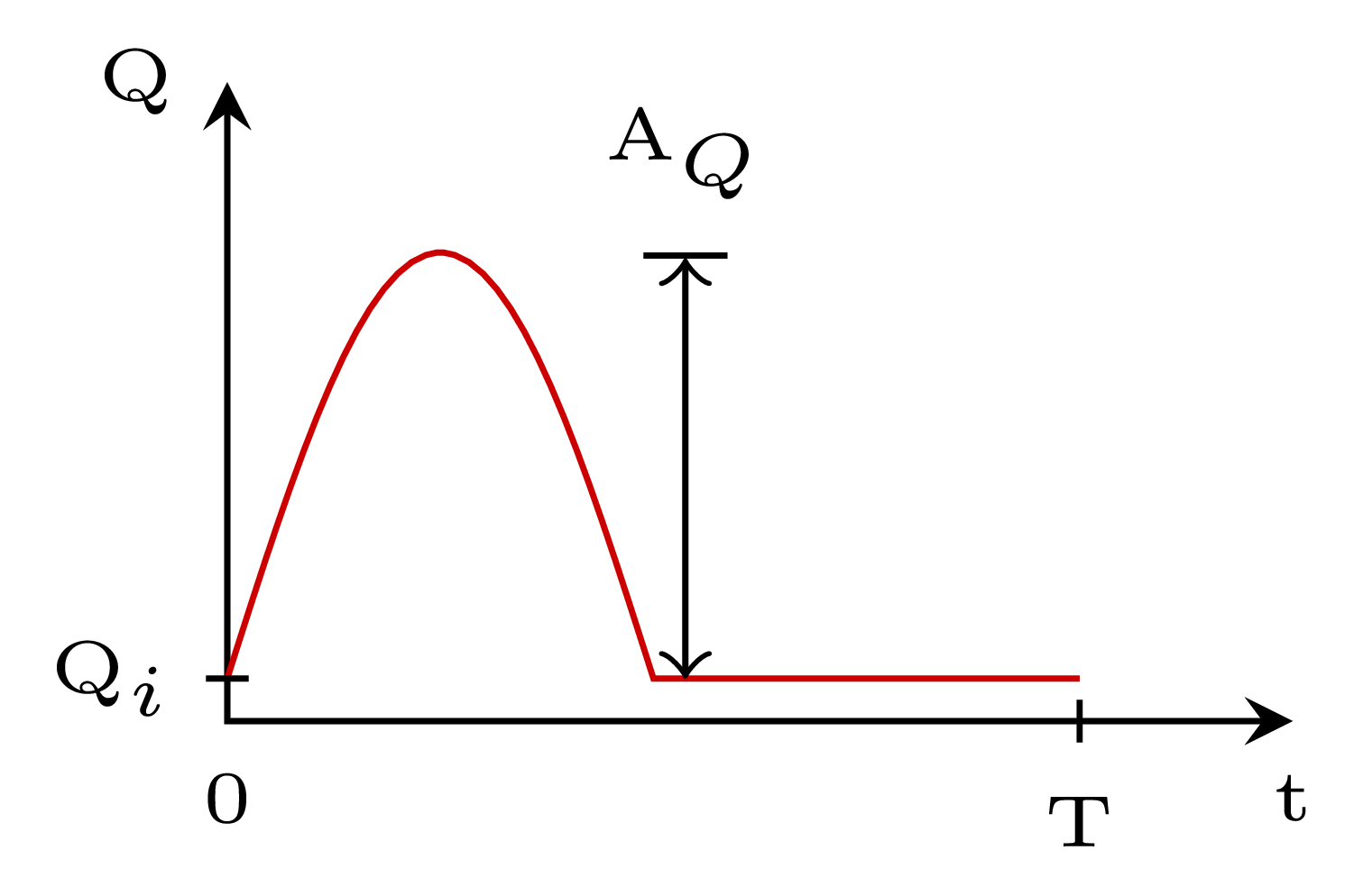
The gaussian bell should span the entire systolic period |
if t < h.sys_T + h.cardiac_T*t_hat && t >= h.cardiac_T*t_hat
|
||||||||||||
|
When this is confirmed, the inlet flow rate reads \[
Q = A_Q \exp{\left(- \frac{\left(t - \hat{t} T -
\tfrac{T_s}{2}\right)^2}{2 \left(\tfrac{T_s}{8}\right)^2 }\right)}
+ Q_i.
\] Variables are the same as those used in |
		return h.flow_amplitude * exp( - (t-t_hat*h.cardiac_T -h.sys_T*0.5)^2 /
            (2*(h.sys_T*0.125)^2)) + initial_flow
|
||||||||||||
|
Otherwise only the
|
	else
		return 0. + initial_flow

	end
end
|
||||||||||||
|
|
|
||||||||||||
|
function
|
function inputFromData(t :: Float64, h :: Heart)
|
||||||||||||
|
	idt = h.input_data[:,1]
	idq = h.input_data[:,2]
|
||||||||||||
|
|
t_hat = div(t,h.cardiac_T)
|
||||||||||||
|
The current time is then updated by subtracting as many cardiac cycles as those already passed. This is done in order to have a reference within the cardiac cycle, i.e. in order to know at what point (when) in the cardiac cycle the simulation is running. |
t -= t_hat*h.cardiac_T
|
||||||||||||
|
The waveform is given in a discrete form and usually with a small amount of points along the cardiac cycle. Usually, the numerical \(\Delta t\) is small enough to fall between two time steps reported in 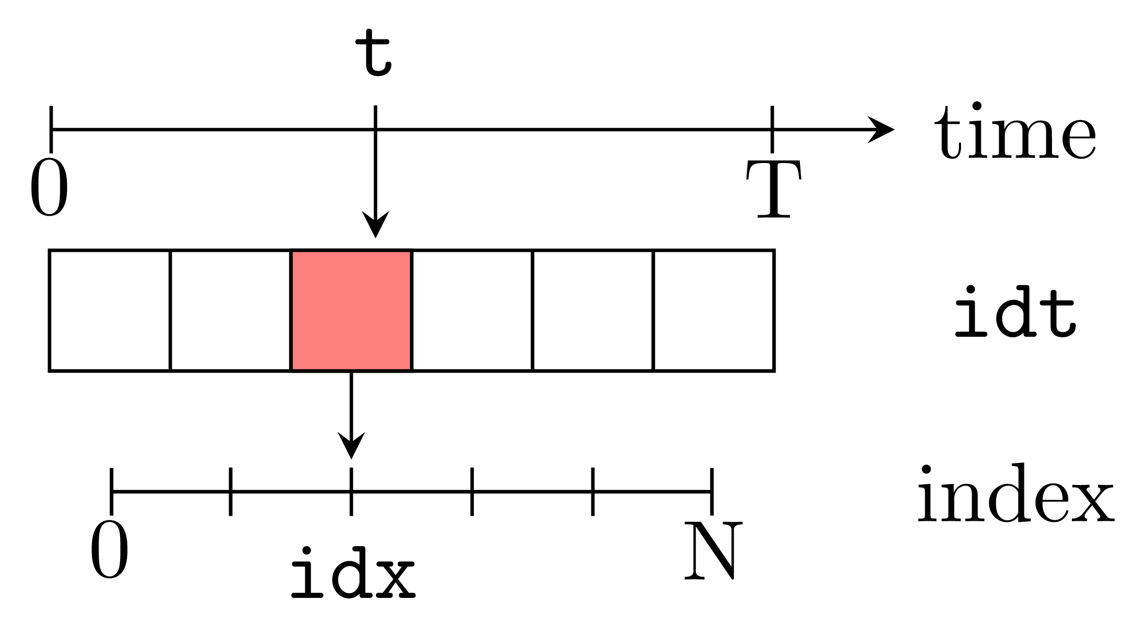
|
	idx = 0
	for i in 1:length(idt)
		if ((t >= idt[i]) && (t <= idt[i+1]))
			idx=i
			break
		end
	end
|
||||||||||||
|
The flow |
	qu = idq[idx] + (t - idt[idx]) * (idq[idx+1] - idq[idx]) /
       (idt[idx+1] - idt[idx])
|
||||||||||||
|
	return qu
end
|
||||||||||||
|
In the case of veins, the inlet is always coupled with three-element Windkessel. The inlet function is re-defined as follows |
|
||||||||||||
|
function
|
function setInletBC(v  :: Vessel,  dt :: Float64,
                    Pc :: Float64, R2 :: Float64)
	v.Q[1] = Pc/R2 + 1e-10

	inletCompatibility(dt, v)
end
|
||||||||||||
|
The inlet compatibility relations are handled by |
|
||||||||||||
|
function
|
function inletCompatibility(dt :: Float64, v :: Vessel, h :: Heart)
|
||||||||||||
|
Riemann invariants are computed starting from variables at time |
	W11, W21 = riemannInvariants(1, v)
	W12, W22 = riemannInvariants(2, v)
|
||||||||||||
|
The two Riemann invariants within the two nodes are extrapolated with a linear law. They reads \[ W_{11}^{t+1} = W_{11}^t + \left(W_{12}^t - W_{11}^t \right) (c_1 - u_1) \frac{\Delta t}{\Delta x}, \] \[ W_{21}^{t+1} = W_{21}^t - W_{11}^{t+1} + 2 \frac{Q_1}{A_1}, \] where the 1 subscript indicates the inlet node. |
	W11 += (W12-W11)*(v.c[1] - v.u[1])*dt/v.dx
	W21 = 2*v.Q[1]/v.A[1] - W11
|
||||||||||||
|
Longitudinal velocity and wave velocity at the inlet node are retrieved by |
v.u[1], v.c[1] = rI2uc(W11, W21)
|
||||||||||||
|
|
	if h.inlet_type == "Q"
		v.A[1] = v.Q[1]/v.u[1]
		v.P[1] = pressure(v.A[1], v.A0[1], v.beta[1], v.Pext)
	else
		v.A[1] = areaFromPressure(v.P[1], v.A0[1], v.beta[1], v.Pext)
		v.Q[1] = v.u[1]*v.A[1]
	end

end

function inletCompatibility(dt :: Float64, v :: Vessel)

	W11, W21 = riemannInvariants(1, v)
	W12, W22 = riemannInvariants(2, v)

	W11 += (W12-W11)*(v.c[1] - v.u[1])*dt/v.dx
	W21 = 2*v.Q[1]/v.A[1] - W11

	v.u[1], v.c[1] = rI2uc(W11, W21)

	v.A[1] = v.Q[1]/v.u[1]
	v.P[1] = pressure(v.A[1], v.A0[1], v.beta[1], v.Pext)

end
|
||||||||||||
|
Outlet boundary condition is applied to the last node of the involved vessel. Two boundary conditions are available. Either a reflection coefficient is provided or a three elements windkessel is coupled. |
|
||||||||||||
|
function
|
function setOutletBC(dt :: Float64, v :: Vessel)
|
||||||||||||
|
A proximal resistance |
	if v.R1 == 0.

		v.P[end] = 2*v.P[end-1] - v.P[end-2]
		outletCompatibility(dt, v)
|
||||||||||||
|
When all the parameters of the three element windkessel are specified, |
	else
		wk3(dt, v)

	end

end
|
||||||||||||
|
Outlet compatibility relations compute all the quantities not directly assigned by the outlet boundary condition. |
|
||||||||||||
|
function
|
function outletCompatibility(dt :: Float64, v :: Vessel)

	W1M1, W2M1 = riemannInvariants(v.M-1, v)
	W1M, W2M   = riemannInvariants(v.M, v)
|
||||||||||||
|
\[ W_{2M}^{t+1} = W_2^t + \frac{W_{2 M-1}^t - W_{2M}^t}{\Delta x} (u_M^t + c_M^t) \Delta t, \] \[ W_{1M}^{t+1} = W_{1M}^0 - R_t \left(W_{2L}^{t+1} - W_{2L}^0 \right). \] |
	W2M += (W2M1 - W2M)*(v.u[end] + v.c[end])*dt/v.dx
	W1M = v.W1M0 - v.Rt * (W2M - v.W2M0)
|
||||||||||||
|
Here the remaining quatities are computed by means of their definitions. |
	v.u[end], v.c[end] = rI2uc(W1M, W2M)
	v.Q[end] = v.A[end]*v.u[end]

end
|
||||||||||||
|
The three element windkessel simulates the perfusion of downstream vessels. This 0D model is coupled by 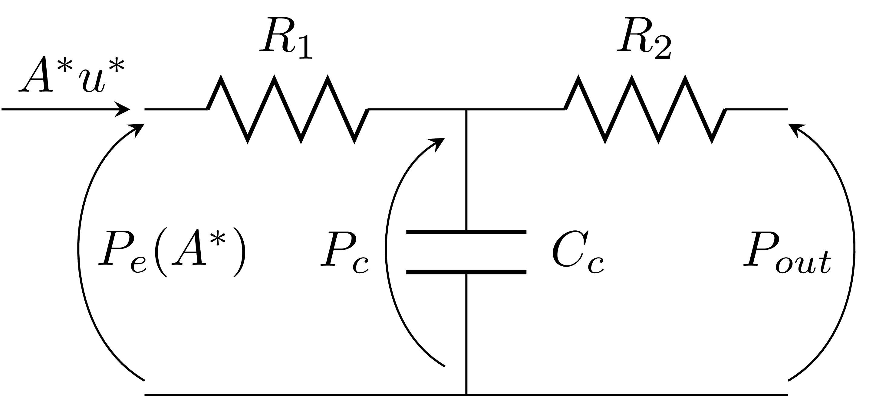
\(R_1\) is the proximal resistance, \(R_2\) is the peripeheral reisistance, \(C_c\) is the peripheral compliance, \(P_c\) is the pressure across the peripheral compliance, \(P_out\) is the pressure at the artery-vein interface, \(P_e\) is the pressure at the 0D/1D interface. |
|
||||||||||||
|
function
|
function wk3(dt :: Float64, v :: Vessel)
|
||||||||||||
|
Pout = 0.
|
||||||||||||
|
The coupling is performed by assuming that an intermediate state \((A^*,u^*)\) generates from \((A_l,u_l)\) (1D outlet) and \((A_r,u_r)\) (0D inlet). This intermediate state must satisfy the windkessel equation \[ A^*u^* \left(1 + \frac{R_1}{R_2}\right) + C_c R_1 \frac{\partial (A^*u^*)}{\partial t} = \frac{P_e - P_{out}}{R_2} + C_c \frac{\partial P_e}{\partial t}. \] |
	Al = v.A[end]
	ul = v.u[end]
|
||||||||||||
|
\(P_c\) is computed at each time step from \[ C_c \frac{\partial P_c}{\partial t} = A^*u^* - \frac{P_c - P_{out}}{R_2}, \] which is discretised numerically with a first-order scheme. \(P_c\) is is initialised to zero. |
v.Pc += dt/v.Cc * (Al*ul - (v.Pc-Pout)/v.R2)
|
||||||||||||
|
We consider \(\beta\) and \(A_0\) to be the same on both sides of the 0D/1D interface. It yields the nonlinear equation \[ \mathcal{F}(A^*) = A^*R_1\left(u_l+4c_l\right) -4A^*R_1c^* - \frac{\beta}{A_0}\left( \sqrt{A^*}-\sqrt{A_0}\right) + P_c = 0, \] where \(c_l\) and \(c^*\) are the wave speeds calculated with \(A_l\) and \(A^*\), respectively. |
As = Al
|
||||||||||||
|
fun(As) = v.R1(ul+4sqrt(3v.gamma[end]sqrt(Al)0.5))As - 4v.R1sqrt(3v.gamma[end]sqrt(As)0.5)As - (v.Pext + v.beta[end]*(sqrt(As/v.A0[end]) - 1)) + v.Pc |
|
||||||||||||
|
dfun(As) = v.R1( ul +4sqrt(1.5v.gamma[end])(sqrt(sqrt(Al)) - 1.25sqrt(sqrt(As))) ) - v.beta[end]0.5/(sqrt(As*v.A0[end])) |
	ssAl = sqrt(sqrt(Al))
	sgamma =  2*sqrt(6*v.gamma[end])
	sA0 = sqrt(v.A0[end])
	bA0 = v.beta[end]/sA0

	fun(As) = As*v.R1*(ul + sgamma * (ssAl - sqrt(sqrt(As)))) -
		(v.Pext + bA0*(sqrt(As) - sA0)) + v.Pc

	dfun(As) = v.R1*(ul + sgamma * (ssAl - 1.25*sqrt(sqrt(As)))) - bA0*0.5/sqrt(As)
|
||||||||||||
|
\(\mathcal{F}(A^*)=0\) is solved for \(A^*\) with the Newton’s method implemented in Roots library. \(A^*\) is initialised equal to \(A_l\). As = newton(fun, dfun, As) |
As = newtone(fun, dfun, As)
|
||||||||||||
|
Once \(A^*\) is found, \(u^*\) reads \[ u^* = \frac{P_e^* - P{out}}{A^*R_1}, \] where \(P_e^*\) is \(P_e\) calculated with \(A^*\). |
	us = (pressure(As, v.A0[end], v.beta[end], v.Pext) - Pout)/(As*v.R1)

	v.A[end] = As
	v.u[end] = us

end

function newtone(f, df, x0)

	xn = x0 - f(x0)/df(x0)
	if abs(xn-x0)<= 1e-5
		return xn
	else
		newtone(f, df, xn)
	end
end
|
||||||||||||
|
function
|
function updateGhostCells(v :: Vessel)

	v.U00A = v.A[1]
	v.U00Q = v.Q[1]
	v.U01A = v.A[2]
	v.U01Q = v.Q[2]

	v.UM1A = v.A[v.M]
	v.UM1Q = v.Q[v.M]
	v.UM2A = v.A[v.M-1]
	v.UM2Q = v.Q[v.M-1]

end
|
||||||||||||
|
|
function updateGhostCells(vessels :: Array{Vessel, 1})

	for vessel in vessels
		updateGhostCells(vessel)
	end

end
|
||||||||||||
References
|
|