godunov.jl

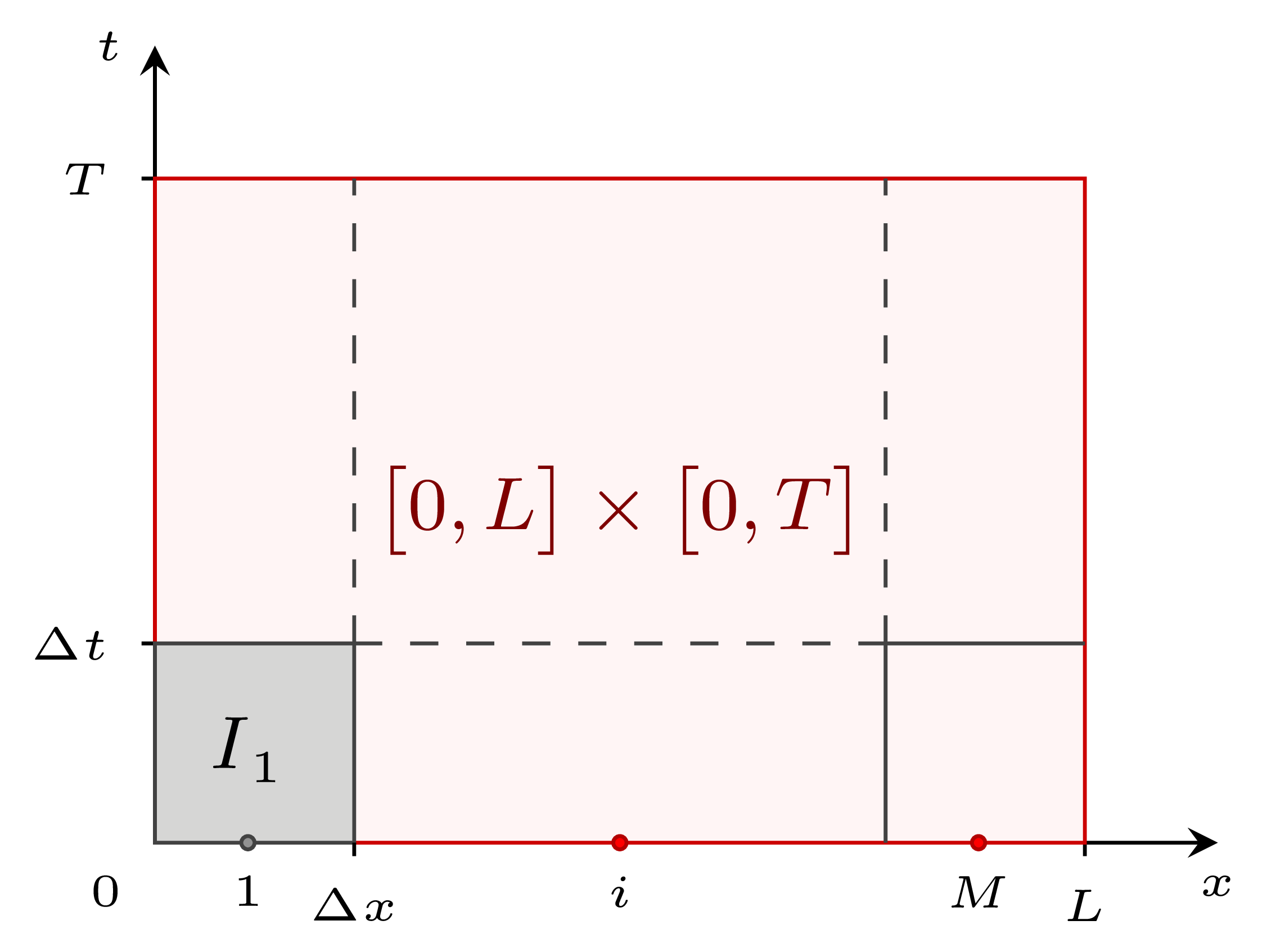
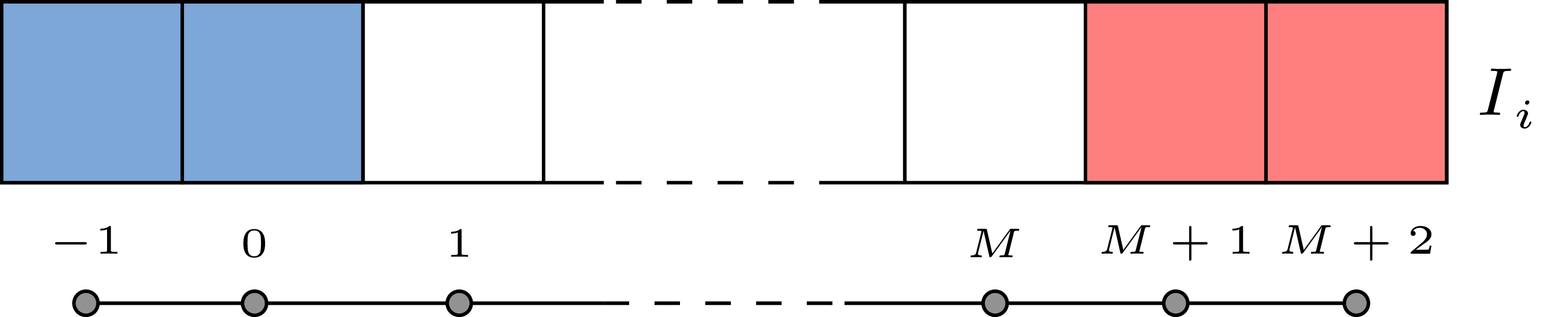
1D blood flow within elastic vessels is ruled by a system of hyperbolic partial derivative equations \[ \begin{cases} \dfrac{\partial A}{\partial t} + \dfrac{\partial Au}{\partial x} = 0, \\ \dfrac{\partial Au}{\partial t} + \dfrac{\partial Au^2}{\partial x} \dfrac{A}{\rho}\dfrac{\partial P}{\partial x} = - Ru, \\ P(x, t) = P_e(x, t) + K_a \left[\left(\dfrac{A}{A_0} \right)^{1/2} -1 \right], \end{cases} \] By defining \(\mathbf{U} = [A, u]^T\), the conservative form of the system can be written along with initial and boundary conditions as \[ \begin{cases} \mathbf{U}_t + \mathbf{F}(\mathbf{U})_x = \mathbf{S}(\mathbf{U}), \quad x \in \big[0, L \big], \\ \mathbf{U}(x, 0) = \mathbf{U}^{(0)}(x), \quad t>0, \\ \mathbf{U}(0, t) = \mathbf{U}_l(t), \mathbf{U}(L, t) = \mathbf{U}_r(t), \end{cases} \] where \(\mathbf{F}\) is the flux term, and \(\mathbf{S}\) is the source term. This set of equations and initial and boundary conditions is also called Initial Boundary Value Problem (IBVP). The IBVP is solved by means of the Godunov’s method ¹, a conservative first order finite volume method. The method is applied on a computational domain (red) subdivided in \(M\) cells \(I_i\) (gray).

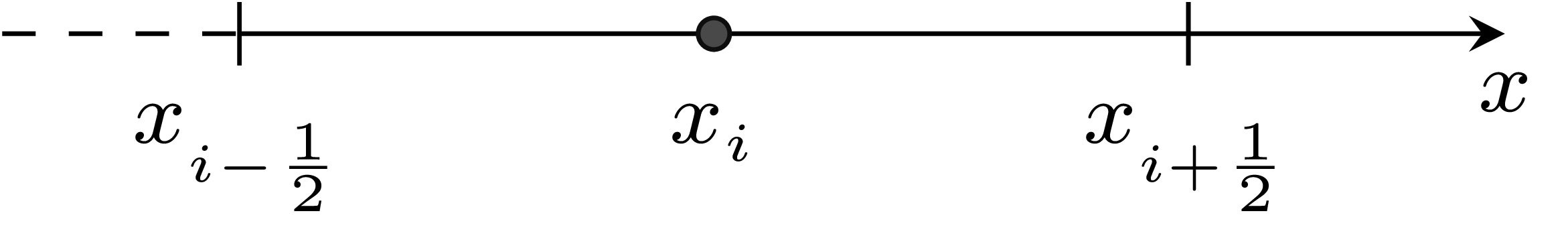
Domain length is equal to vessel length \(L\), and cell length is given by \(\Delta x\) size. The total simulation time \(T\) defines domain height, hence cell height is given by \(\Delta t\). In each cell \(I_i\) three points are defined: center point \(x_i\), left extreme \(x_{i-1/2}\), and right extreme \(x_{i+1/2}\).

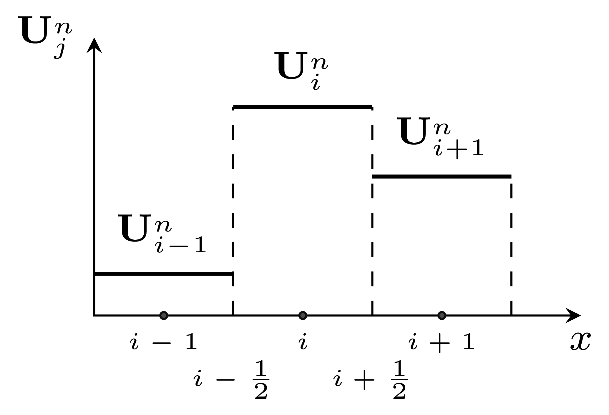
Godunov’s method assumes a piece-wise constant distribution of \(\mathbf{U}\) at each \(t = t^n\).

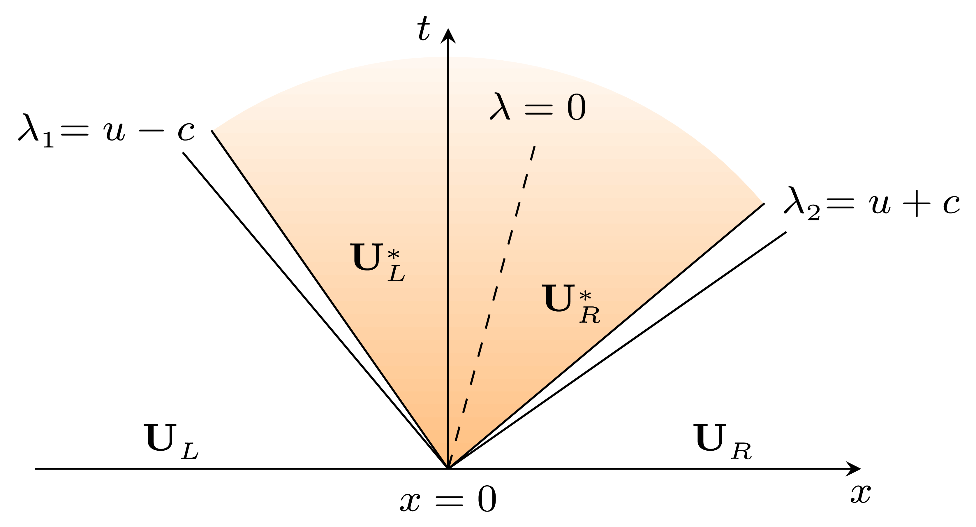
For a small enough \(\Delta t\), the method updates the solution as \[ \mathbf{U}_i^{n+1} = \mathbf{U}_i^{n} + \frac{\Delta t}{\Delta x} \left(\mathbf{F}_{i-1/2} - \mathbf{F}_{i+1/2} \right), \] where \(\mathbf{F}_{i\pm 1/2} = \mathbf{F}\left(\mathbf{U}_{i\pm 1/2}(0) \right)\) is the numerical flux. The argument of the numerical flux, \(\mathbf{U}_{i\pm 1/2}(0)\), is computed as the solution of a homogeneous ( the source term will be added later on) quasi-linear local Riemann problem (RP) at the interface of two cells. For \(\mathbf{U}_{i + 1/2}(0)\) we have \[ \begin{cases} \mathbf{U}_t + \mathbf{F}_\mathbf{U} \mathbf{U}_x = 0, \\ \mathbf{U}(x_i, 0) = \mathbf{U}^{(0)}(x_i) = \begin{cases} \mathbf{U}_L = \mathbf{U}(x_{i-1/2}), \quad x<0, \\ \mathbf{U}_R = \mathbf{U}(x_{i+1/2}), \quad x>0. \\ \end{cases} \end{cases} \] The solution of the RP is depicted below.

The solution structure includes two families of waves associated to the two system Riemann invariants \(\lambda_1\) and \(\lambda_2\), respectively. There are three constant states \(\mathbf{U}_L\), \(\mathbf{U}^*\), and \(\mathbf{U}_R\), of which \(\mathbf{U}^*\) is unknown and refers to the solution in the star region (yellow). We need jump conditions to cross the waves and connect these states. Depending on the nature of each wave we have shock or rarefaction conditions.

Godunov function glues together all the functions needed to solve the RP at each interface and to compute the numerical flux.

function Godunov

First we compute the states \(\mathbf{U}_L\) and \(\mathbf{U}_R\) at the left hand side interface (\(i-1/2\)). When we deal with the inlet node (\(i=1\)), blue ghost cells are used to find left states. Right states are always inside the numerical domain and they do not need ghost cells.

Once the local states have been computed, the solution of the RP at the left interface is found by riemannSolver function.

The same process is applied to the local right interface.

When both interfaces are solved, left and right (\(\mathbf{F}_{i\mp 1/2}\)) numerical fluxes are computed by flux fucntion.

Conservative variables A and Q are updated by Godunov’s method formula.

The source term is solved by source function and Q is directly updated. The source term is always zero for the continuity equation, hence A is not updated.

Eventually, primitive variables P, u, and c are updated accordingly to their definitions by pressure and waveSpeed functions.

The RP solution is herein coded. The Riemann solver computes the cross-sectional area in the star region \(A^*\) starting from a guess solution (two rarefactions solution). The value of \(A^*\) comes from the solution of the nonlinear equation \[ f(A^*) = f_L(A^*) + f_R(A^*) + \Delta u = 0, \] where \(\Delta u = u_R - u_L\), and \(f_L\) and \(f_R\) are the local fluxes computed by fl and fr, respectively.

function riemannSolver \(\rightarrow\) As::Float, Qs::Float

The nonlinear equation for the RP is defined and solved by Newton’s method.

Eventually, \(u^*\) is computed as \[ \frac{1}{2}\left(u_L + u_R\right) + \frac{1}{2}\left[f_R\left(A^*\right) -f_L\left(A^* \right) \right], \]

\(Q^*\) is calculated from its definition and returned.

Local fluxes (left and right) are computed depending on the nature of the wave system located at the interface. In particular \[ f_L = \begin{cases} 4\left(c^* - c_L\right), & A^*\leq A_L \quad \text{(rarefaction)}, \\ \sqrt{\dfrac{\gamma\left(A^*-A_L\right)\left(A^{* 3/2}- A_L^{3/2}\right)}{A_L A^*}}, & A^*>A_L \quad \text{(shock)}, \end{cases} \] \[ f_R = \begin{cases} 4\left(c^* - c_R\right), & A^*\leq A_R \quad \text{(rarefaction)}, \\ \sqrt{\dfrac{\gamma\left(A^*-A_R\right)\left(A^{* 3/2}- A_R^{3/2}\right)}{A_R A^*}}, & A^*>A_R \quad \text{(shock)}, \end{cases} \]

function fL \(\rightarrow\) left_flux::Float

function fR \(\rightarrow\) right_flux::Float

The flux in conservative form reads \[ \mathbf{F}(\mathbf{U}) = \left\{ \begin{array}{c} Au \\ Au^2 + \gamma A^{3/2} \end{array} \right\}, \] and its numerical form is computed by flux function.

function flux \(\rightarrow\) f1::Float, f2::Float

function source \(\rightarrow\) S::Float

function calculateDeltaT \(\rightarrow\) DT::Float

For each vessel the \(\Delta t\) is computed as \[ \Delta t = \frac{\Delta x}{S_{max}} C_{cfl} \] where \(S_{max}\) is the maximum between the forward and the backward characteristics, and \(C_{cfl}\) is the Courant-Friedrichs-Lewy condition defined by the user.

function solveModel

References